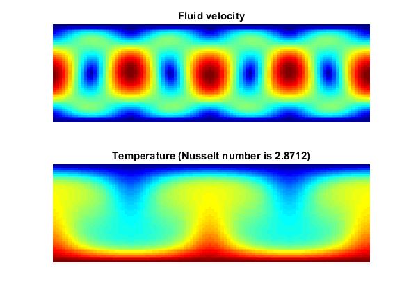
From:
https://palabos.unige.ch/get-started/lattice-boltzmann/lattice-boltzmann-sample-codes-various-other-programming-languages/
%%%%%%%%%%%%%%%%%%%%%%%%%%%%%%%%%%%%%%%%%%%%%%%%%%%%%%
% thermalLB.m: Rayleigh Benard Convection, using a LB method,
% based on [Z.Guo, e.a., http://dx.doi.org/10.1002/fld.337].
% Boussinesq approximation is used for the buoyancy term:
% - Fluid is approximated with incompressible Navier-Stokes
% equations including a body force term, and simulated
% with a BGK model
% - Temperature is approximated with advection-diffusion
% equation and simulated with a BGK model
%
%%%%%%%%%%%%%%%%%%%%%%%%%%%%%%%%%%%%%%%%%%%%%%%%%%%%%%
% Lattice Boltzmann sample, written in matlab
% Copyright (C) 2008 Andrea Parmigiani, Orestis Malaspinas, Jonas Latt
% Address: Rue General Dufour 24, 1211 Geneva 4, Switzerland
% E-mail: andrea.parmigiani@terre.unige.ch
%%%%%%%%%%%%%%%%%%%%%%%%%%%%%%%%%%%%%%%%%%%%%%%%%%%%%%
% This program is free software; you can redistribute it and/or
% modify it under the terms of the GNU General Public License
% as published by the Free Software Foundation; either version 2
% of the License, or (at your option) any later version.
% This program is distributed in the hope that it will be useful,
% but WITHOUT ANY WARRANTY; without even the implied warranty of
% MERCHANTABILITY or FITNESS FOR A PARTICULAR PURPOSE. See the
% GNU General Public License for more details.
% You should have received a copy of the GNU General Public
% License along with this program; if not, write to the Free
% Software Foundation, Inc., 51 Franklin Street, Fifth Floor,
% Boston, MA 02110-1301, USA.
%%%%%%%%%%%%%%%%%%%%%%%%%%%%%%%%%%%%%%%%%%%%%%%%%%%%%%
clear
% GENERAL FLOW CONSTANTS
ly = 51;
aspect_ratio = 2;
lx = aspect_ratio*ly;
delta_x = 1./(ly-2);
Pr = 1.;
Ra = 20000.; % Rayleigh number
gr = 0.001; % Gravity
buoyancy = [0,gr];
Thot = 1; % Heating on bottom wall
Tcold = 0; % Cooling on top wall
T0 = (Thot+Tcold)/2;
delta_t = sqrt(gr*delta_x);
% nu: kinematic viscosity in lattice units
nu = sqrt(Pr/Ra)*delta_t/(delta_x*delta_x);
% k: thermal diffusivity
k = sqrt(1./(Pr*Ra))*delta_t/(delta_x*delta_x);
omegaNS = 1./(3*nu+0.5); % Relaxation parameter for fluid
omegaT = 1./(3.*k+0.5); % Relaxation parameter for temperature
maxT = 80000; % total number of iterations
tPlot = 100; % iterations between successive graphical outputs
tStatistics = 10; % iterations between successive file accesses
% D2Q9 LATTICE CONSTANTS
tNS = [4/9, 1/9,1/9,1/9,1/9, 1/36,1/36,1/36,1/36];
cxNS = [ 0, 1, 0, -1, 0, 1, -1, -1, 1];
cyNS = [ 0, 0, 1, 0, -1, 1, 1, -1, -1];
oppNS = [ 1, 4, 5, 2, 3, 8, 9, 6, 7];
% D2Q5 LATTICE CONSTANTS
tT = [1/3, 1/6, 1/6, 1/6, 1/6];
cxT = [ 0, 1, 0, -1, 0];
cyT = [ 0, 0, 1, 0, -1];
oppT = [ 1, 4, 5, 2, 3];
[y,x] = meshgrid(1:ly,1:lx);
% INITIAL CONDITION FOR FLUID: (rho=1, u=0) ==> fIn(i) = t(i)
fIn = reshape( tNS' * ones(1,lx*ly), 9, lx, ly);
% INITIAL CONDITION FOR TEMPERATURE: (T=0) ==> TIn(i) = t(i)
tIn = reshape( tT' *Tcold *ones(1,lx*ly), 5, lx, ly);
% Except for bottom wall, where T=1
tIn(:,:,ly)=Thot*tT'*ones(1,lx);
% We need a small trigger, to break symmetry
tIn(:,lx/2,ly-1)= tT*(Thot + (Thot/10.));
% Open file for statistics
fid = fopen('thermal_statistics.dat','w');
fprintf(fid,'Thermal Statistics: time-step --- uy[nx/2,ny/2] --- Nu\n\n\n');
% MAIN LOOP (TIME CYCLES)
for cycle = 1:maxT
% MACROSCOPIC VARIABLES
rho = sum(fIn);
T = sum(tIn); %temperature
ux = reshape ( (cxNS * reshape(fIn,9,lx*ly)), 1,lx,ly) ./rho;
uy = reshape ( (cyNS * reshape(fIn,9,lx*ly)), 1,lx,ly) ./rho;
% MACROSCOPIC BOUNDARY CONDITIONS
% NO-SLIP for fluid and CONSTANT at lower and upper
% boundary... periodicity wrt. left-right
% COLLISION STEP FLUID
for i=1:9
cuNS = 3*(cxNS(i)*ux+cyNS(i)*uy);
fEq(i,:,:) = rho .* tNS(i) .* ...
( 1 + cuNS + 1/2*(cuNS.*cuNS) - 3/2*(ux.^2+uy.^2) );
force(i,:,:) = 3.*tNS(i) .*rho .* (T-T0) .* ...
(cxNS(i)*buoyancy(1)+cyNS(i)*buoyancy(2))/(Thot-Tcold);
fOut(i,:,:) = fIn(i,:,:) - omegaNS .* (fIn(i,:,:)-fEq(i,:,:)) + force(i,:,:);
end
% COLLISION STEP TEMPERATURE
for i=1:5
cu = 3*(cxT(i)*ux+cyT(i)*uy);
tEq(i,:,:) = T .* tT(i) .* ( 1 + cu );
tOut(i,:,:) = tIn(i,:,:) - omegaT .* (tIn(i,:,:)-tEq(i,:,:));
end
% MICROSCOPIC BOUNDARY CONDITIONS FOR FLUID
for i=1:9
fOut(i,:,1) = fIn(oppNS(i),:,1);
fOut(i,:,ly) = fIn(oppNS(i),:,ly);
end
% STREAMING STEP FLUID
for i=1:9
fIn(i,:,:) = circshift(fOut(i,:,:), [0,cxNS(i),cyNS(i)]);
end
% STREAMING STEP FLUID
for i=1:5
tIn(i,:,:) = circshift(tOut(i,:,:), [0,cxT(i),cyT(i)]);
end
% MICROSCOPIC BOUNDARY CONDITIONS FOR TEMEPERATURE
%
tIn(5,:,ly) = Tcold-tIn(1,:,ly)-tIn(2,:,ly)-tIn(3,:,ly)-tIn(4,:,ly);
tIn(3,:,1) = Thot-tIn(1,:,1) -tIn(2,:,1) -tIn(4,:,1) -tIn(5,:,1);
% VISUALIZATION
if (mod(cycle,tStatistics)==0)
u = reshape(sqrt(ux.^2+uy.^2),lx,ly);
uy_Nu = reshape(uy,lx,ly); % vertical velocity
T = reshape(T,lx,ly);
Nu = 1. + sum(sum(uy_Nu.*T))/(lx*k*(Thot-Tcold));
fprintf(fid,'%8.0f %12.8f %12.8f\n',cycle,u(int8(lx/2),int8(ly/2))^2, Nu);
if(mod(cycle,tPlot)==0)
subplot(2,1,1);
imagesc(u(:,ly:-1:1)');
title('Fluid velocity');
axis off; drawnow
subplot(2,1,2);
imagesc(T(:,ly:-1:1)')
title(['Temperature (Nusselt number is ' num2str(Nu) ')']);
axis off; drawnow
end
end
end
fclose(fid);

